Penalty/Barrier functions for controls¶

U_COS_LOGARITHMIC¶

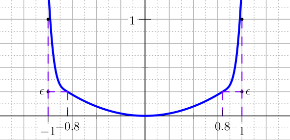
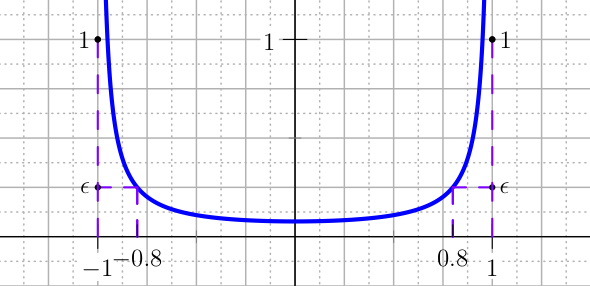
An elegant barrier is the cosine-logarithmic barrier function. To keep the control in \(I\) and avoid values outside that interval, without limiting the freedom of the solver, the cosine-logarithmic barrier for the interval \(I=[a,b]\) is defined as:

\[\chi_I(x) \approx p(x) = -c\ln\cos\left(\dfrac{\pi}{2}\cdot\dfrac{2x-(b+a)}{b-a}\right)\]

with \(c\) such that \(p(x)\) evaluated at \(x=b-\delta\) or \(a+\delta\) takes the value \(\mathbf{a}repsilon\). Where \(\delta=\mathrm{tol}(b-a)/2\) and \(\mathrm{tol}\) is a tolerance and \(\mathbf{a}repsilon\in(0,1)\).

The value \(\mathrm{tol}\) is the distance from the border of \(I\) and \(\mathbf{a}repsilon\) is the value assumed by \(p\) at that point.

They are therefore useful to control the shape of the function. In particular, notice that inside \(I\) the values of \(p\) are very small, while for \(x\) outside \(I\) the cosine becomes negative, hence the logarithm is complex.

The default values are \(\mathrm{tol}=0.001\) and \(\mathbf{a}repsilon=0.001\). To fix the ideas consider the following example, let \(I=[-1,3]\) and the values \(\mathrm{tol}=0.25\) and \(\mathbf{a}repsilon=0.5\).

Then \(\delta=\mathrm{tol}(b-a)/2=0.5\) and the corresponding scaling parameter \(c\) becomes \(c=0.52053\ldots\), see Figure The plot of the cosine logarithmic barrier with the parameters discussed in the example..

Because the manual setting of \(\delta\) and \(c\) is not straightforward (although easy), the user can setup the related values \(\mathrm{tol}\) and \(\mathbf{a}repsilon\) and the others will be computed automatically.

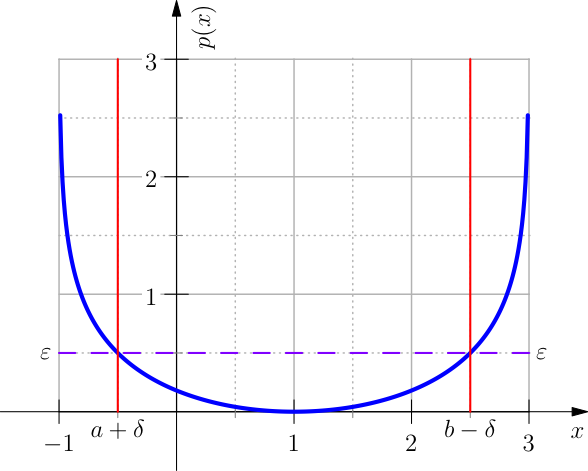
The plot of the cosine logarithmic barrier with the parameters discussed in the example.¶

The command addControlBound will output many informations: the name of the control, by default uControl, the type of the class (penalty, barrier), the control itself \(u(\zeta)\), its range, an eventual scaling factor, the tolerances of the penalty (epsilon and tolerance), the type of the penalty (in this example the cosine-logarithmic).

> addControlBound(
  u,
  controlType = "U_COS_LOGARITHMIC",
  max = -1, min = 3
);

Added the following penalty constraint
  name      = uControl
  class     = PenaltyBarrierU
  u         = u(zeta)
  [min,max] = [-1,3]
  scale     = 1
  epsilon   = .1e-2 (*)
  tolerance = .1e-2 (*)
  type      = U_COS_LOGARITHMIC
  (*) can be changed when using continuation

U_QUADRATIC¶

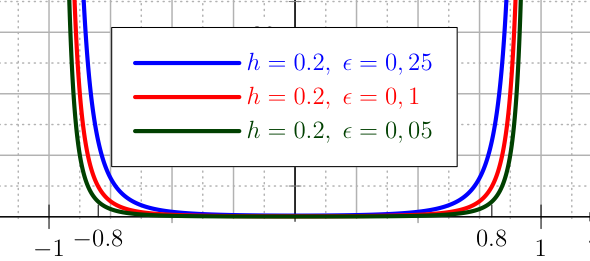
An easy type of penalty for the control is the U_QUADRATIC. The standard formulation is defined over \([-1,1]\), but a change of scale is done automatically in the user defined range \([a,b]\). Here the standard case is presented. Chose the tolerances \(\epsilon\) and \(h\) as depicted in Figure The plot of the U_QUADRATIC penalty for the control.,

The plot of the U_QUADRATIC penalty for the control.¶

and define the auxiliary constants

\[H:= 1-h, \qquad A_1:= \dfrac{\epsilon}{H^2}, \qquad A_2=\dfrac{H^2-\epsilon}{H^2h^2}.\]

Then the penalty is defined as

\[\begin{split}p(x)= A_1x^2+A_2 \begin{cases} (x+H)^2 & \mbox{ if } x\leq -H\\[1em] 0 & \mbox{ if } x\in (-H,H)\\[1em] (x-H)^2 & \mbox{ if } x\geq H \end{cases}\end{split}\]

The first and second derivatives are shown in Figure The plot of the first derivatives of the U_QUADRATIC penalty for the control. and are not smooth.

The plot of the first derivatives of the U_QUADRATIC penalty for the control.¶

The plot of thesecond derivatives of the U_QUADRATIC penalty for the control.¶

U_QUADRATIC_BIS¶

A more advanced penalty than the quadratic presented in U_QUADRATIC is called U_QUADRATIC_BIS, which is defined in terms of the same two tolerances \(\epsilon\) and \(h\), see Figure The plot of the U_QUADRATIC_BIS penalty for the control.. The definition of this penalty is

The plot of the U_QUADRATIC_BIS penalty for the control.¶

\[\begin{split}p(x) := \begin{cases} 1+(2\,A_0(x+1)-A_4)(x+1) & x < -1 \\[1em] \epsilon + ( A_3(x+H) - A_2)(x+H) & x\in[-1,-1+h] \\[1em] A_1\, x^2 & x\in[-H,H] \\[1em] \epsilon + ( A_3(x-H) + A2)(x-H) & x\in[H,1] \\[1em] 1 + ( 2A_0 (x-1) + A_4 )(x-1) & x>1, \end{cases}\end{split}\]

where

\[\begin{split}H := 1-h,\quad A_0 := \frac{1}{h},\qquad A_1 := \frac{\epsilon}{H^2}, \\ A_2 := \frac{2\epsilon}{H}, \qquad A_3 := \frac{1-A_1+h^2A_1}{h^2}+A_1, \qquad A_4 := \frac{2\left(1-A_1\right)}{h}+ A_2.\end{split}\]

The first and second derivative of this penalty are shown in Figure The plot of the first derivatives of the U_QUADRATIC_BIS penalty for the control..

The plot of the first derivatives of the U_QUADRATIC_BIS penalty for the control.¶

The plot of the second derivatives of the U_QUADRATIC_BIS penalty for the control.¶

U_CUBIC¶

The U_CUBIC penalty exhibits a steeper growth than the quadratic penalties, in fact it is modelled by a cubic polynomial. Moreover, increasing the degree of the polynomial it is possible to obtain a smoother function in terms of its derivatives. The shape of the penalty is governed by the usual two tolerances \(\epsilon\) and \(h\) (see Figure The plot of the U_CUBIC penalty for the control.), the definition of the U_CUBIC penalty is:

The plot of the U_CUBIC penalty for the control.¶

\[\begin{split}p(x) = \begin{cases} 1+(A_5\,(x+1)-A_4)(x+1) & x < -1 \\[1em] \epsilon + ((A_2-A_3(x+H))(x+H)-A_1)(x+H) & x\in[-1,-H] \\[1em] A_2\, x^2 & x\in[-H,H] \\[1em] \epsilon + ((A_2+A_3(x-H))(x-H)+A_1)(x-H) & x\in[H,1] \\[1em] 1+(A_5\,(x-1)+A_4)(x-1) & x>1, \end{cases}\end{split}\]

where the auxiliary constants are computed to guarantee continuity of the function and a smooth first derivative, the second derivative is not smooth. They are:

\[H = 1-h,\quad A_1 = \frac{2\epsilon}{H},\quad A_2 = \frac{\epsilon}{H^2},\quad A_3 = \frac{1-A_2}{h^3},\]

\[A_4 = \frac{3(1-A_2)}{h}+2A_2,\quad A_5 = \frac{3(1-A_2)}{h^2}+A_2,\quad A_6 = A_2^2-3A_1A_3\]

The plot of the first and second derivative are shown in Figure The plot of the first derivatives of the U_CUBIC penalty for the control.

The plot of the first derivatives of the U_CUBIC penalty for the control.¶

The plot of the second derivatives of the U_CUBIC penalty for the control.¶

U_QUARTIC¶

In the same fashion of the previous penalties, the U_QUARTIC works in the same way but using a quartic polynomial. This implies a very steep growth and a smooth second derivative. But a problem with those quick growths is given by numerical problems when using a Newton method, e.g. the value becomes quickly a NaN or the iteration gives a point outside of the desired interval. Therefore the user has to be careful and not increasing the degree of the polynomial blindly to have a smoother function.

The definition of the U_QUARTIC penalty (see Figure The graph of the U_QUARTIC penalty with its first and second derivative.}) is

\[\begin{split}p(x) = \epsilon\frac{x^2}{H^2} + \frac{1}{H^4} \begin{cases} (x+H)^4 & x < -1+h \\[1em] 0 & x\in[-H,H] \\[1em] (x-H)^4 & x > 1-h, \end{cases}\end{split}\]

where \(H=1-h\) and \(\epsilon\) together with \(h\) are the parameters that control the shape of the function. The first two derivatives of U_QUARTIC are shown in Figure The graph of the U_QUARTIC penalty with its first and second derivative.}.

The graph of the U_QUARTIC penalty with its first and second derivative.}¶

U_PARABOLA¶

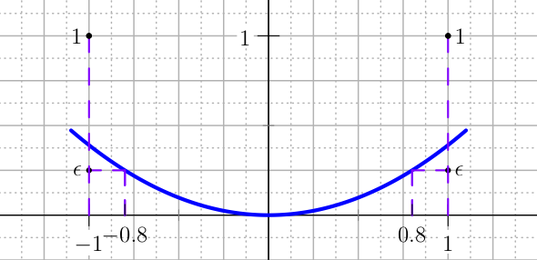
The penalty U_PARABOLA is very simple, and is defined by

\[p(x)=Cx^2,\]

where \(C\) is a constant dependent of the two tolerances \(h\) and \(\epsilon\). It is defined as \(C=\frac{\epsilon}{(1-h)^2}\), so that the penalty assumes value \(\epsilon\) for \(x=\pm(1-h)\), see Figure The graph of the U_PARABOLA penalty with its first and second derivative. for the function and its derivatives.

The graph of the U_PARABOLA penalty with its first and second derivative.¶

U_LOGARITHMIC ————0

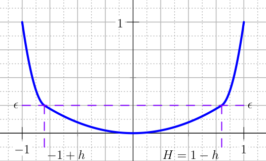
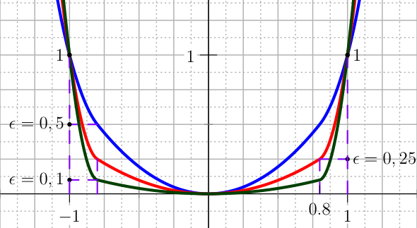
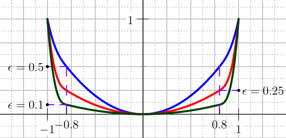
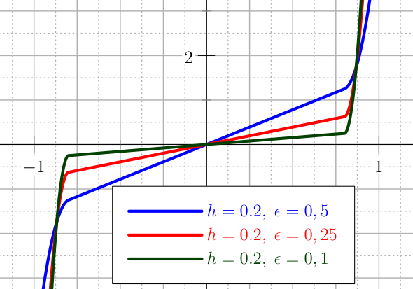
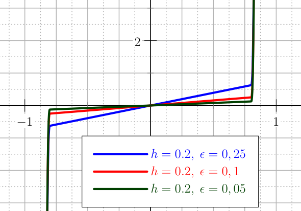
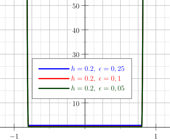
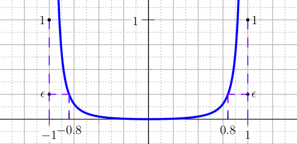
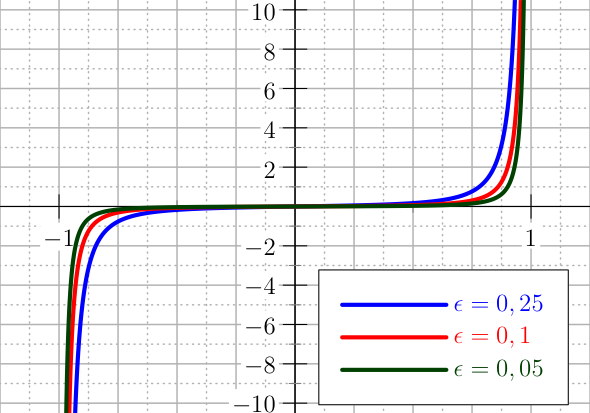
Putting aside the polynomials and looking at transcendental functions, the logarithm is a powerful tool. The barrier U_LOGARITHMIC forces the control in the specified interval, while the penalties allow the control to be outside the interval during the numeric solution process, and ensure at the end that the optimal control is in the correct interval. For the interval \([-1,1]\) the barrier U_LOGARITHMIC is defined as (see Figure The plot of the barrier U_LOGARITHMIC for the control.):

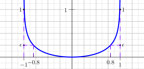
The plot of the barrier U_LOGARITHMIC for the control.¶

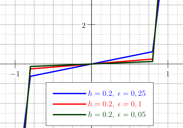
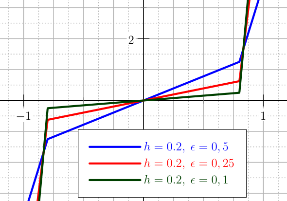
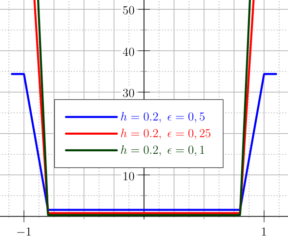
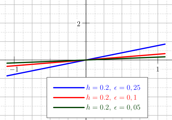
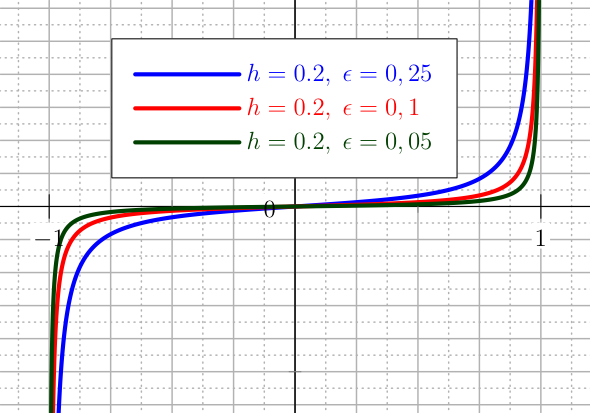
\[p(x)= C \ln (1-x^2), \qquad C:= \dfrac{\epsilon}{\ln(h(2-h))},\]

where \(h\) and \(\epsilon\) are the tolerances fixed by the user so that \(p(1-h)=\epsilon\). The plot of the first and second derivative of this barrier is given in Figure The plot of the first derivatives of the barrier U_LOGARITHMIC for the control..

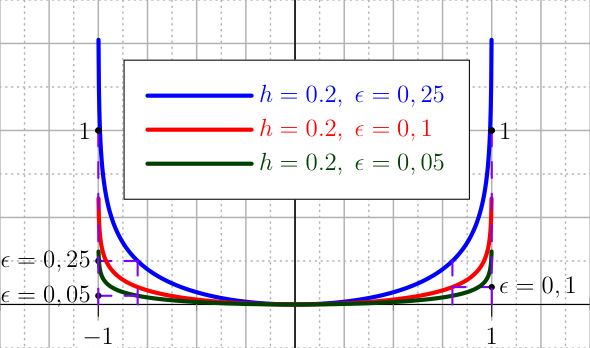
The plot of the first derivatives of the barrier U_LOGARITHMIC for the control.¶

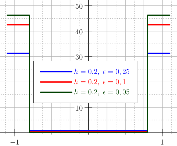
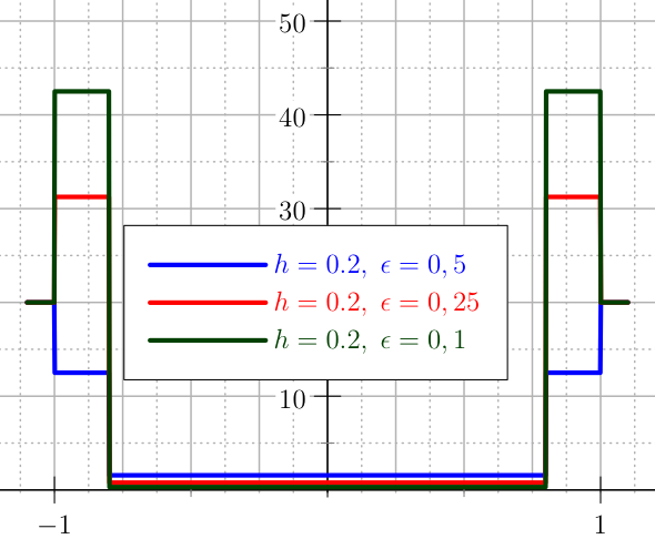
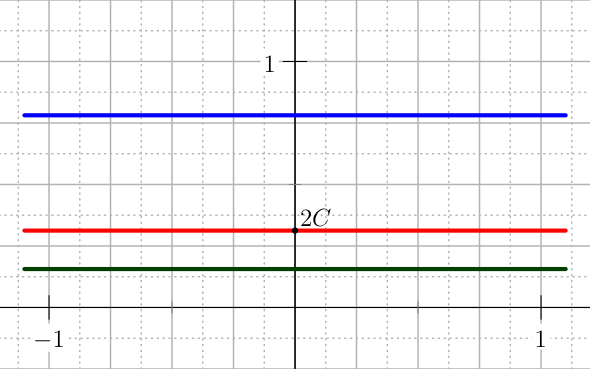
The plot of the second derivatives of the barrier U_LOGARITHMIC for the control.¶

U_TAN2¶

Another kind of barrier is given by a manipulation of the tangent function, namely, for the interval \([-1,1]\):

\[p(x):= C \left[\tan \frac{\pi x}{2}\right]^2, \qquad C:= \dfrac{\epsilon}{\left[\tan \frac{\pi (1-h)}{2}\right]^2 }.\]

The coefficient \(C\) is dependent of the two tolerances \(h\) and \(\epsilon\) and is computed so that \(p(1-h)=\epsilon\), see Figure The graph of the U_TAN2 penalty with its first and second derivative. for the function and its derivatives.

The graph of the U_TAN2 penalty with its first and second derivative.¶

U_HYPERBOLIC¶

Another trigonometric barrier is given by a manipulation of the hyperbolic function, namely, for the interval \([-1,1]\):

\[p(x):= \dfrac{C}{\cos \frac{\pi x}{2}}, \qquad C:= \epsilon \cos \frac{\pi (1-h)}{2}.\]

The coefficient \(C\) is dependent of the two tolerances \(h\) and \(\epsilon\) and is computed so that \(p(1-h)=\epsilon\), see Figure The graph of the U_HYPERBOLIC penalty with its first and second derivative. for the function and its derivatives.

The graph of the U_HYPERBOLIC penalty with its first and second derivative.¶

U_BIPOWER¶

A penalty which is the juxtaposition of two polynomials of different degree is the U_BIPOWER. It is defined as the convex combination of the monomial \(x^2\) and \(x^N\):

\[p(x):= \delta x^2 + (1-\delta) x^N\]

The coefficient \(\delta\) is dependent of the two tolerances \(h\) and \(\epsilon\) and \(N\in\mathbb{N}\) is the first even integer such that

\[N \geq \dfrac{\ln \frac{\epsilon}{2}}{\ln (1-h)}.\]

Coefficient \(\delta\) is computed so that

\[\delta = \frac{\epsilon-(1-h)^N}{(1-h)^2-(1-h)^N} \geq \frac{\epsilon}{2}.\]

See Figure The graph of the U_BIPOWER penalty with its first and second derivative. for the function and its derivatives.

The graph of the U_BIPOWER penalty with its first and second derivative.¶