Quick Start
How to set up an ODE
How to set up an OCP: Quick Start for Beginners
In this section an incremental set of examples for preparing an OCP is presented.
The first example is the classic bang-bang mass, the basic instructions for a quick start are introduced.
The next examples will add more and more features in
order to give a sufficiently deep insight in pins.
For a more detailed description, refer to the next chapters
where the single commands of XOptima are listed.
Example 1: Fixed Time Bang Bang
In PINS each problem must have a name,
for this first tutorial choose for simplicity
‘’Fixed_Time_Bang_Bang’’.
The best thing to do is to create on a desired
location the folder
Fixed_Time_Bang_Bang and the subfolder model.
Inside that subfolder create an open a Maple worksheet called
Fixed_Time_Bang_Bang.mw, this will contain all the
necessary instruction for XOptima to define the
OCP and generate the optimised C++ code for Mechatronix
that will be run by pins.
The situation in your folder should be the one
depicted in Figure:

The folder tree for the first start with pins.
You are now ready to define the OCP! Suppose to solve the following OCP: maximise 1 the distance of a classic bang-bang mass starting at the origin and standing at rest at the final point. The time interval is fixed in \([0,T]\) with \(T=1\). The equations of the problem are:
- 1
-
Please notice that XOptima only minimises the functional, in order to maximise it add a minus sign as in ((1))
The first thing to do in Maple is to load the XOptima Library with the command
> with(XOptima):
Module '     XOptima', Copyright (C) B-cube Team ...
Module ' XOptimaPars', Copyright (C) B-cube Team ...
Module ' XOptimaSUBS', Copyright (C) B-cube Team ...
This will display information of the version of XOptima and the credits, of course now you have loaded the package. The next step is to define the states and controls. The corresponding variables are \(x(t)\), \(v(t)\) - position and velocity - and \(u(t)\) the control.
> qvars := [x(t),v(t)] ;
> cvars := [u(t)] ;
Having defined the variables, it is possible to define the dynamical system by specifying the differential equations:
> EQ1 := diff(x(t),t) = v(t) ;
> EQ2 := diff(v(t),t) = u(t) ;
With the next instruction the dynamical system is given to XOptima:
> loadDynamicSystem(
  equations = [EQ1,EQ2],
  controls  =  cvars,
  states    =  qvars
);
This instruction will output the message ‘’Independent variable \(t\) has been redefined to \(\zeta\)’’ and the confirm of the state variables in \(\zeta\). Now you can select which boundary conditions are active, in this case the initial conditions for \(x\) and \(v\) and the final condition on \(v\), then you can specify explicitly that \(x(0)=0\), \(v(0)=0\), \(v(T)=0\).
> addBoundaryConditions(
  initial = [x = 0,v = 0],
  final   = [v = 0]
);
This is done with the help of a penalty function. There are many types of penalties, they are described more in detail later. For now use a general penalty that works most of the times, the cosine-logarithmic penalty (see Figure The plot of the cosine logarithmic barrier with the parameters discussed in the example. and Chapter Interface of XOptima):
> addControlBound(
  u,
  controlType = "U_COS_LOGARITHMIC",
  max = 1, min = -2
);
the command should return the message:
Added the following penalty constraint
name      = uControl
class     = PenaltyBarrierU
u         = u(zeta)
[min,max] = [-2,1]
scale     = 1
epsilon   = .1e-2 (*)
tolerance = .1e-2 (*)
type      = U_COS_LOGARITHMIC
(*) can be changed when using continuation
To have an idea of what this penalty does, consider for simplicity the interval \(I=(a,b)\). Penalty and barrier functions are function that smoothly approximates the characteristic function \(\chi_I(x)\) that is identically zero inside \(I\) and infinity outside \(I\). The problem is that the discontinuity cannot be treated numerically in the convergence process. Hence it is convenient to find a smooth function that approximates the discontinuity.
A barrier function is a smooth functions with takes infinity value outside the interval \(I\), while a penalty function is defined in the whole space while is fastly growing outside the interval \(I\). There are many of those functions available in XOptima, an elegant one is the cosine-logarithmic barrier function. To keep the control in \(I\) and avoid values outside that interval, without limiting the freedom of the solver, the cosine-logarithmic barrier for the interval \(I=[a,b]\) is defined as:
with \(c\) such that \(p(x)\) evaluated at \(x=b-\delta\) or \(a+\delta\) takes the value \(\varepsilon\). Where \(\delta=\mathrm{tol}(b-a)/2\) and \(\mathrm{tol}\) is a tolerance and \(\varepsilon\in(0,1)\). The value \(\mathrm{tol}\) is the distance from the border of \(I\) and \(\varepsilon\) is the value assumed by \(p\) at that point. They are therefore useful to control the shape of the function.
In particular, notice that inside \(I\) the values of \(p\) are very small, while for \(x\) outside \(I\) the cosine becomes negative, hence the logarithm is complex. The default values are \(\mathrm{tol}=0.001\) and \(\varepsilon=0.001\).
This command will output many informations: the name
of the control, by default uControl,
the type of the class (penalty, barrier),
the control itself \(u(\zeta)\), its range,
an eventual scaling factor, the tolerances
of the penalty (epsilon and tolerance),
the type of the penalty (in this example the cosine-logarithmic).
All those quantities are described better later,
for this introductory example every parameter
is set by default.
To specify the target (that is another name for the functional to be optimised, another used name is performance index) you can choose to write it as a Mayer term or as Lagrange 2 term. You can select both possibilities:
- 2
-
It is always possible to convert among Mayer problems, Lagrange problems and Bolza problems
> setTarget( lagrange = 0, mayer = -x(zeta_f) ) ;
# or equivalently setTarget( mayer = -x(zeta_f) ) ;
Added target definition
  Lagrange term = -v(zeta)
  Mayer term    = 0
which selects the minimisation of the Mayer term
To setup the classic Lagrange term
> setTarget( lagrange = -v(zeta), mayer = 0 ) ;
# or equivalently setTarget( lagrange = -v(zeta) ) ;
Added target definition
  Lagrange term = 0
  Mayer term    = -x(zeta_R)
Please notice the presence of the subscript _f for the final point of the Mayer term. Similarly, for an initial point there is the subscript _i. Although mathematically the two formulations are equivalent, the use of the Lagrange term or the Mayer term will produce (slight) numerical differences.
The setup process is complete, the last thing to do
is to tell XOptima to produce the C++ code
for the optimal control problem.
At this stage you can specify a guess function for the
solution, this will improve dramatically the solution process.
The command generateOCProblem is the most important
in XOptima because it allows to specify
many numerical properties and features
(e.g. the use of continuation). In this example it
is used in the minimal way.
In the next examples more properties will follow.
For now consider
> generateOCProblem(
  "Fixed_Time_Bang_Bang",
  mesh         = [ length=1, n=100 ],
  states_guess = [ x=0, v=0 ]
);
Step 1, generate BVP
--------------------
Generating list of variables
Building penalty functions (Jp_fun)
Building Hamiltonian function (H_fun)
Building gradient of Hamiltonian function (dHdx_vec)
Building dinamical system with co-equation
Building system of equations of optimal controls (g_vec)
Building left and right substitution for jump and boundary conditions
Building equations of boundary conditions (BC_fun, BC_vec)
Building equations for interface or transition conditions

Step 2, solve or guess controls
-------------------------------
       .
       .
       .

Code generation completed!
--------------------------
Deleting unnecessary files!
where
“Fixed_Time_Bang_Bang”is the name of the project and of the generated C++ object.meshsets the length of the interval for the independent variable and number of nodesstates_guessfor a guess of the states, in this case not very clever as \(x\equiv 0\) and \(v\equiv 0\).
The previous command will generate the C++ and Ruby
code to be linked with Mechatronix and run with pins.
It is convenient to rewrite the Maple code for the
first example Fixed_Time_Bang_Bang/model/Fixed_Time_Bang_Bang.mw
in a unique listing:
> # Begin Fixed_Time_Bang_Bang in XOptima
> restart:
> with(XOptima):
> qvars := [x(t),v(t)];
> cvars := [u(t)];
> EQ1 := diff(x(t),t) = v(t);
> EQ2 := diff(v(t),t) = u(t);
> loadDynamicSystem(
    equations = [EQ1,EQ2],
    controls  = cvars,
    states    = qvars
  );
> addBoundaryConditions(
    initial = [x = 0,v = 0],
    final   = [v = 0]
  );
> addControlBound(
    u,
    controlType = "U_COS_LOGARITHMIC",
    max = 1, min = -2
  );
> setTarget( lagrange = -v(zeta), mayer = 0 ) ;
> generateOCProblem(
    "Fixed_Time_Bang_Bang",
    mesh         = [ length=1, n=100 ],
    states_guess = [ x=0, v=0 ]
  );
> # End of Fixed_Time_Bang_Bang in XOptima
Having run the the Maple sheet, you should find in the
Fixed_Time_Bang_Bang folder the tree of files of
Figure The folder tree for the first start with PINS after the code generation and the run of the executable..
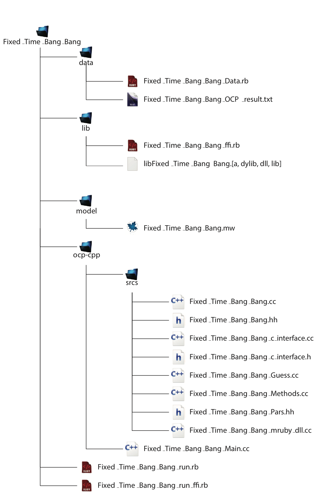
The folder tree for the first start with PINS after the code generation and the run of the executable.
To compile and run the code, open a console and surf
to the main folder Fixed_Time_Bang_Bang.
Then simply type
$ pins Fixed_Time_Bang_Bang_run.rb -f
This will compile, link and run the project, to only run it type
$ pins Fixed_Time_Bang_Bang_run.rb
The final screenshot, after listing of the iterations, will look like
STATISTICS
N. equations  =    407    Iter                  = 14
MaxIter       =    300    tolerance             = 1e-09
lambdaMin     =  1e-20    last residual         = 1.925e-16
lambdaDump    =      2    last ``new'' residual = 1.126e-10
Elapsed Time  =  179.4ms  last ||f||_1          = 1.208e-11


numMeritFunctionEvaluation = 0
numFunctionEvaluation      = 62
numMultiplyByJacobian      = 0
numJacobianFactorization   = 14
numJacobianInversion       = 75
  ______                                          _
 / _____)                                        | |
| /      ___  ____ _   _ ____  ____ ____  ____ _ | |
| |     / _ \|  _ \ | | / _  )/ ___) _  |/ _  ) || |
| \____| |_| | | | \ V ( (/ /| |  ( ( | ( (/ ( (_| |
 \______)___/|_| |_|\_/ \____)_|   \_|| |\____)____|
                                  (_____|
Here you can have some statistics and other informations
about the computational time, number of itarations,
number of operations in terms of evaluations,
inversions etc. The numerical results are stored in
a plain text file, called Data/Fixed_Time_Bang_Bang_OCP_result.txt
(have a look at Figure The folder tree for the first start with PINS after the code generation and the run of the executable.).
In the results files are reported the evaluations of the
functions and variables of the OC problem for each node pointwise.
In Figure The folder tree for the first start with PINS after the code generation and the run of the executable. is given the typical
structure of the directories of the generated files.
The first folder Data contains a text file .rb
that stores the parameters of the optimal control problem.
This is useful if you want to solve several instances of
the OCP tuning manually some constants.
Modify the Ruby script and you do not have to recompile
the C++ project, but simply rerun the executable.
In this folder you find also the text file of the results,
XOptima will append the string NOT_CONVERGED
to the file name if the execution of the code does not converge.
In the folder lib there are the compiled files of the library
with the ffi interface for Ruby: if you are using Windows
there will be two libraries, a file .lib and a .dll;
under Linux a file nfile{.a} and under Mac OSX a file .dylib.
In the directory model there is the source
code of your problem in XOptima.
The corresponding source code for
Mechatronix generated and optimised in
C++ is contained in the folder ocp-cpp,
where you can find the main executable,
and in the subfolder srcs there are the header files,
the interfaces to C and to Ruby, the source
files for the user defined functions.
All those files are automatically created by
XOptima when you run the command generateOCProblem.
Numerical results
The solution of the classic bang-bang example (1) is \(J^\star=x(T)=\frac{1}{3}\) and
The plot of the results given by PINS is reported in Figure fig1.
|
|
|


For the same example done in ACADO, please refer to the Appendix.
Example 2: Free Time and fixed distance
This second example incrementally introduces a new feature expanding the previous example. The fixed time constraint is removed and a fixed distance to travel is introduced. The OCP is to minimise the time taken to travel from a rest position in the origin to the point at distance \(L=10\). The original mathematical formulation is:
To solve a minimum time problem in PINS it is necessary to reformulate it in fixed time, this is done introducing an extra variable, the final time \(T\). The differential equation corresponding to variable \(T\) is obviously \(T^\prime=0\) because the final time is constant. Therefore the problem is defined by three variables \(x\), \(v\), \(T\) and three equations. The independent variable can be set to \(\zeta\) (a kind of time). The original equations of (2) must be multiplied by the factor \(T(\zeta)\) accordingly to the change of variable (for more details on those changes, refer to Minimum Time):
This first part is coded in XOptima in the same way of the previous example and is:
> restart:
> with(XOptima):
> qvars := [x(zeta), v(zeta), T(zeta)];
> cvars := [u(zeta)];
> EQ1 := diff(x(zeta),zeta) = T(zeta)*v(zeta);
> EQ2 := diff(v(zeta),zeta) = T(zeta)*u(t);
> EQ2 := diff(T(zeta),zeta) = 0;
> loadDynamicSystem(
  equations = [EQ1,EQ2,EQ3],
  controls  =  cvars,
  states    =  qvars
);
The boundary conditions are also straightforward to set, also the control does not change:
> addBoundaryConditions(initial = [x=0,v=0],final=[v=0,x=L]);
> addControlBound(
  u, controlType="U_COS_LOGARITHMIC",
  max=1, min=-2, scale = T(zeta)
);
Notice that the value \(L\) is defined but not
initialised yet. All the parameters and constant
are defined together inside the command
generateOCProblem at the end of the file.
The last part of the script is intuitive and resembles the previous example, it is only matter to define the target, the constants such as the value of \(L=10\) and a guess to help the solver. It is all done with the next two commands
> setTarget( lagrange = 0, mayer = T(zeta_f) ) ;
> generateOCProblem(
  "Free_Time_Fixed_Distance",
  parameters         = [ L = 10 ],
  mesh               = [ length=1, n=100 ],
  states_guess       = [ x=L*zeta, v=0, T=1 ],
  admissible_regions = [ T(zeta)>0 ]
);
To solve the problem numerically,
it is necessary to specify that the final time
\(T\) can not be negative, because clearly a
negative time has no physical meaning in this context.
This is easily achieved by setting a check on the
\(T\) variable with the option admissible_regions.
Again, it is not necessary to conceive a particularly exotic guess, here the three variables are approximated with something reasonable, but it is valuable to point out that a good guess can be effective in the convergence process for complex and structured problems, therefore an at least basic physical knowledge of the problem is important. For conveniency, the complete script for the second example is reported next.
> # Begin of Free_Time_Fixed_Distance in XOptima

> restart:
> with(XOptima):
> qvars := [x(zeta), v(zeta), T(zeta)];
> cvars := [u(zeta)];
> EQ1 := diff(x(zeta),zeta) = T(zeta)*v(zeta);
> EQ2 := diff(v(zeta),zeta) = T(zeta)*u(t);
> EQ2 := diff(T(zeta),zeta) = 0;
> loadDynamicSystem(
  equations = [EQ1,EQ2,EQ3],
  controls  =  cvars,
  states    =  qvars
);

> addBoundaryConditions(initial = [x=0,v=0],final=[v=0,x=L]);

> addControlBound(
  u, controlType="U_COS_LOGARITHMIC",
  max=1, min=-2, scale = T(zeta)
);

> setTarget( lagrange = 0, mayer = T(zeta_f) );

> generateOCProblem(
  "Free_Time_Fixed_Distance",
  parameters         = [ L = 10 ],
  mesh               = [ length=1, n=100 ],
  states_guess       = [ x=L*zeta, v=0, T=1 ],
  admissible_regions = [ T(zeta)>0 ]
);

> # End of Free_Time_Fixed_Distance in XOptima
The plot of the results given by PINS is reported in Figure:
|
|
|


The exact solution, for a comparison, is quite similar to the previous exercise, the switching point is placed at \(\zeta=\frac{2}{3}\) and the minimum time is \(T^\star=\sqrt{30}\approx 5.47\). The exact solutions of the optimal trajectory and control are:
Example 3: Free Time and fixed distance with two controls
The natural expansion of the previous example is the introduction of two controls, namely the two pedals of the brake \(b(t)\) and of the throttle \(p(t)\), also the fuel mass is taken into account. The controls are antagonists, but it is interesting to see that the optimal solution admits a time interval in which both are saturating. The original problem is a minimum time OCP:
\[\begin{split}\begin{array}{rl} \textrm{minimize: }& T \\[1em] \textrm{ subject to }& x^\prime(t)=v(t), \quad m(t)v^\prime(t)=p(t)-b(t), m^\prime(t)=-k_2p(t); \\[1em] & x(0)=0, v(0)=0, m(0)=m_0, v(T)=0, x(T)=L; \\[1em] & \qquad p(t)\in [0,1],\quad b(t)\in [0,2],\quad t\in[0,T]. \end{array}\end{split}\]
The coefficient of fuel consumption is \(k_2=0.2\), the initial mass is \(m_0=1\), the fixed distance to reach is \(L=10\). As seen before, the problem must be firstly converted in a fixed time problem, this is done simply by adding the new (constant) variable \(T\) and the relative change of variable that transforms problem eqref{QS:ocp:example3} in:
\[\begin{split}\begin{array}{rl} \textrm{minimize: }& T \\[1em] \textrm{ subject to }& x'(\zeta)=T(\zeta)v(\zeta), \quad m(\zeta)v'(\zeta)=T(\zeta)(p(\zeta)-b(\zeta)),\\ & m'(\zeta)=-k_2T(\zeta)p(\zeta), \quad T'(\zeta)=0; \\[1em] & x(0)=0, v(0)=0, m(0)=m_0, v(1)=0, x(1)=L; \\[1em] & \qquad p(\zeta)\in [0,1],\quad b(\zeta)\in [0,2],\quad \zeta\in[0,1]. \end{array}\end{split}\]
The plots of the numerical solution of the problem are depicted in Figure:
|
|
|
|
|
|


This is coded directly in XOptima as follows:
> # Begin of Free_Time_Fixed_Distance_Two_Controls in XOptima
> restart:
> with(XOptima):
> qvars := [x(zeta), v(zeta), m(zeta), T(zeta)];
> cvars := [p(zeta), b(zeta)];
> EQ1 := diff(x(zeta),zeta) = T(zeta)*v(zeta);
> EQ2 := m(zeta)*diff(v(zeta),zeta) = T(zeta)*(p(zeta)-b(zeta));
> EQ3 := diff(m(zeta),zeta) = -T(zeta)*k2*p(zeta);
> EQ4 := diff(T(zeta),zeta) = 0;

> loadDynamicSystem(
  equations = [EQ1,EQ2,EQ3,EQ4],
  controls  =  cvars,
  states    =  qvars
);

> addBoundaryConditions( initial = [x=0,v=0,m=m0],final=[v=0,x=L]);

> addControlBound(
  p, controlType="U_COS_LOGARITHMIC",
  max=1, min=0, scale=T(zeta)
);

> addControlBound(
  b, controlType="U_COS_LOGARITHMIC",
  max=2, min=0, scale=T(zeta)
);

> setTarget( lagrange = 0, mayer = T(zeta_f) );

> generateOCProblem(
   "Free_Time_Mass_Consumption",
   parameters         = [ L = 10, m0=1, k2 = 0.2 ],
   mesh               = [ length=1, n=100 ],
   states_guess       = [ x=L*zeta, v=L, T=1, m = m0 ],
   admissible_regions = [ T(zeta)>0, m(zeta)>0, v(zeta)>=0 ]
);

> # End of Free_Time_Fixed_Distance_Two_Controls in XOptima
Example 4: Free Time and Interface Conditions, a pit stop
The next expansion of the original example is the minimum
time problem of the mass with a fixed distance to travel,
the push and brake controls, mass consumption and a pit
stop to refill the fuel. There are more constraints:
the mass (fuel) should not go below a minimum value
\(m\geq m_0=1\), the pit stop should last a non
negative time interval called \(S(\zeta)\)
(but coded as pitstop for clearness)
and has to be done at half the way, at \(x=L/2=50\).
During the pit stop, the fuel enters the tank at the
speed of \(\delta_m=0.1\).
The target is the total time taken from the origin to \(L\), it is the sum of the time needed to travel the first segment until the pit stop plus the time required to fill the fuel plus the time needed for the second stint to the final point. The variable \(T\) will be modelled as a piecewise constant function, that will give the time for the two segments. For simplicity it is added the variable \(t(\zeta)\) (coded as inlX{tm}) which models the true time over the two segments (plus the pit stop) and is the integral of \(T\).
The dynamical system, after the conversion from free time to fixed time with the change of variable seen so far, is:
\[\begin{split}\begin{array}{rl} \textrm{minimize: }& t(\zeta_f)\\[1em] \textrm{ subject to }& x^\prime(\zeta)=T(\zeta)v(\zeta), \quad m(\zeta)v^\prime(\zeta)=T(\zeta)(p(\zeta)-b(\zeta)),\\ & m^\prime(\zeta)=-k_2T(\zeta)p(\zeta),\quad S^\prime(\zeta)=0,\\ & t^\prime(\zeta)=T(\zeta), \quad T^\prime(\zeta)=0; \\[1em] & x(0)=0,\; v(0)=0,\; m(0)=m_0+f,\;t(0)=0,\\[1em] & v(1)=0,\; x(1)=L,\; m(1)=m_0; \\[1em] & \qquad p(\zeta)\in [0,1],\quad b(\zeta)\in [0,2],\quad \zeta\in[0,1]. \end{array}\end{split}\]
This first part of the description of the OCP becomes in XOptima:
> restart:
> with(XOptima):
> qvars := [x(zeta), v(zeta), m(zeta), pitstop(zeta), tm(zeta), T(zeta)];
> cvars := [p(zeta), b(zeta)] ;

> EQ1 := diff(x(zeta),zeta) = T(zeta)*v(zeta) ;
> EQ2 := m(zeta)*diff(v(zeta),zeta) = T(zeta)*(p(zeta)-b(zeta)) ;
> EQ3 := diff(m(zeta),zeta) = -T(zeta)*k2*p(zeta) ;
> EQ4 := diff(pitstop(zeta),zeta) = 0 ;
> EQ5 := diff(tm(zeta),zeta) = T(zeta) ;
> EQ6 := diff(T(zeta),zeta)  = 0 ;

> loadDynamicSystem(
  equations = [EQ||(1..6)],
  controls  =  cvars,
  states    =  qvars
);

> addBoundaryConditions(
  initial=[x=0,v=0,m=m0+fuel,tm=0],
  final  =[v=0,x=L,m=m0]
);
The bounds of the problem, apart from the controls \(p\) and \(b\) limited respectively in \([0,1]\) and \([0,2]\), are the minimum length of the pit stop set to \(s(\zeta)\geq 1\) and the mass limit, \(m(\zeta)\geq m_0\).
Other bounds that are useful to be added to the problem in order to avoid non natural solutions like negative times are \(T(\zeta)>0\), \(v(\zeta)\geq 0\), \(m(\zeta)\geq 0\) and \(s(\zeta)\geq 0\).
It becomes clear even to the inexperienced reader that the constraints and the equations start to get involved and this will bring numerical problems. Without a very precise guess and a lot of numerical expertise it is possible to help the solver to go to convergence. This is clearly non always the case.
A better way to reach convergence to the desired accuracy is to use the technique of continuation, which is a concept close to the idea of homotopy. A more precise definition is given later in the present manual, for now, an intuitive explanation and the usage are given. The idea is to create a sequence of OCPs, starting from an easy one (from a numeric point of view) towards the hardest one (the desired OCP).
This process is first split into continuation steps, and each step allows a parameter of transformation. To fix the ideas, suppose to consider only one step and consider to transform the tolerances of the penalty functions. If those tolerances are very strict the solver will have problems to converge, if they are too loose, the solver converges easily but the solution will be of low interest, e.g. the corners where the control jumps are not very sharp
The key idea of the continuation is to create a sequence of OCPs with changing parameter, in this case the tolerances of the penalties. Each solution is used as a good guess for the next OCP of the sequence. There is a parameter of transformation that brings down the value of the tolerances from a big value to the desired one. When convergence with that value is achieved, a new step of the continuation process is performed. The presence of this feature is a strong point of XOptima and allows to solve very complex problems as it will shown in the section of advanced problems.
It is time to turn the attention to how to
implement in the XOptima code the continuation.
It is the user that has to decide on which parameters
to apply the continuation and on how many steps.
For this example it is enough to create a single
step and to transform the values of the tolerances
of the penalties, the values of epsilon and of tolerance.
It is convenient to choose two values, a maximum and
a minimum for both, as constant parameters at the
end of the program when you call generateOCProblem,
hence respectively epsi0, epsi1 and
tol0, tol1.
The values epsi0 and tol0 represent the loose
values to start the sequence of continuation problems.
XOptima will automatically choose the transformation
parameter \(s\in[0,1]\), starting from 0 and
reaching 1, that will solve the final OCP
with tolerances set to epsi1 and tol1.
In practise, those constraints are coded as:
> addControlBound(
  p, controlType="U_COS_LOGARITHMIC", max=1, min=0,
  scale=T(zeta), epsilon=epsi0, tolerance=tol0
);

> addControlBound(
  b, controlType="U_COS_LOGARITHMIC", max=2, min=0,
  scale=T(zeta), epsilon=epsi0, tolerance=tol0
);

> addUnilateralConstraint(
  pitstop(zeta) >= 1, "minimumPitStop",
  barrier=false, scale = T(zeta),
  epsilon=epsi0, tolerance=tol0
);

> addUnilateralConstraint(
  m(zeta) >= m0, "massLimit",
  barrier=false, scale = T(zeta),
  epsilon=epsi0, tolerance=tol0
);
Typical values for those tolerances can be \(0.1\)
and \(0.0001\) for epsi0 and epsi1 respectively;
\(0.01\) and \(0.001\) for tol0 and tol1.
The default value for epsi1 and tol1 is \(0.001\).
You can now specify and set the target:
> setTarget( mayer = tm(zeta_f) );
Up to here there is nothing new, what makes this example different from the previous is the presence of internal constraints: the important feature of this example is the presentation of the interface conditions. They represent the behaviour of the dynamical system in particular points inside the integration interval. In this case the interface is constituted by the behaviour at the pit stop: the mass changes because of the refuelling, the particle must arrive at the pit stop with zero velocity, stand still for all the pit stop operations and then leave.
> setInterfaceConditionAlgebraic( [
     m(zeta_R)       = m(zeta_L) + pitstop(zeta_L)*dm,
     tm(zeta_R)      = tm(zeta_L) + pitstop(zeta_L),
     pitstop(zeta_R) = pitstop(zeta_L)
  ] );
> setInterfaceConditionFree( T );
> setInterfaceConditionFixed( x, x(zeta_L)=L/2, x(zeta_R)=L/2 );
> setInterfaceConditionFixed( v, v(zeta_L)=0, v(zeta_R)=0 );
Notice that it is not known when (i.e. the time instant)
the pit stop takes place, but only that it is located halfway
at \(x=L/2\). This condition is expressed with the
command setInterfaceConditionFixed,
the fact that the position does not change is expressed
with the two equations \(x(\zeta_L) = L/2\) and
\(x(\zeta_R) = L/2\), where \(\zeta_L\) and
\(\zeta_L\) are the values of the independent
variable (pseudotime) before and after the pit stop.
To specify that the time \(T\) is piecewise constant
over the two segments, use the command setInterfaceConditionFree.
What happens during the pit stop is modelled with the
instruction setInterfaceConditionAlgebraic,
here the mass augments because of the refuelling process,
which is a linear function of the pit stop time,
that is, after the pit stop (\(m(\zeta_R)\)),
the mass is \(m(\zeta_L)+s(\zeta_L) \delta_m\).
The variable \(s\) is actually a constant
(the pit stop time), hence it must be the same before
and after the pit stop, which is modelled with
the equation \(s(\zeta_R)= s(\zeta_L)\).
The final part of this example is to specify the parameters of the problem (constants, coefficients, continuation, guesses) and generate the code. It is convenient to save the specifications of the continuation in a single variable:
> CONTINUATION := [[
  ["p","epsilon"]                = epsi0 + s*(epsi1-epsi0),
  ["p","tolerance"]              = tol0  + s*(tol1-tol0),
  ["b","epsilon"]                = epsi0 + s*(epsi1-epsi0),
  ["b","tolerance"]              = tol0  + s*(tol1-tol0),
  ["minimumPitStop","epsilon"]   = [epsi0,epsi1],
  ["minimumPitStop","tolerance"] = [tol0,tol1],
  ["massLimit","epsilon"]        = [epsi0,epsi1],
  ["massLimit","tolerance"]      = [tol0,tol1]
]];
The previous line is a list of lists, each element
of the main list is a step of the continuation process,
as said before, in this example there is only one step
and hence one element.
Inside this element you can specify on which parameters
you want to perform the transformation process from
tol0 to tol1 and similarly with epsi0
and epsi1.
The syntax is easy: each element of the transformation
process is a list that contains the name of the object,
its parameter and an expression,
e.g.~``epsi0+s*(epsi1-epsi0)``.
This last expression is equal to epsi0
at the beginning of the transformation (i.e. for \(s=0\))
and to epsi1 when the step is completed
(i.e. for \(s=1\)).
Please notice that you cannot choose the name
of the variable \(s\) inside the expression
epsi0+s*(epsi1-epsi0) and that the choice of
the value of \(s\in[0,1]\) is done by XOptima
during the solution.
Notice also the shortcut [epsi0,epsi1]
instead of the expression epsi0+s*(epsi1-epsi0):
they are exactly the same and represent a
linear interpolation of the two values.
To tell XOptima to use the continuation
just add the command in generateOCProblem.
The final part of the code is therefore:
> generateOCProblem(
  "Free_Time_Pit_Stop",
  parameters   = [ L=100, m0=1, k2=0.02, dm=0.1, Tsize=10, f=0.1*m0,
                   epsi0=0.1, epsi1=0.0001,
                   tol0 =0.01, tol1=0.001],
  mesh         = [ [length=0.5, n=250],[length=0.5, n=250] ],
  continuation = CONTINUATION,
  states_guess = [ x=zeta*L, v=L/Tsize, T=Tsize, m=m0,
                   tm=zeta*Tsize, pitstop = 1 ],
  admissible_regions = [ T(zeta)>0, m(zeta)>=0, v(zeta)>=0, pitstop(zeta) >= 0 ]
);
Notice that the mesh can be specified for each segment of the problem, the guesses are reasonable and a rule of the thumb is to furnish a linear interpolation of the initial and final conditions (when available). The plots of the numerical solution of the problem are depicted in Figure The numerical solution obtained with the code described in Section chap:QS:sec:ex4, with, respectively, the states x, v, m and the optimal controls p and b and the optimal time t(1)\approx 43.91. The pit stop time is around 1.59..
|
|
|
|
|
|


From the plots of Figure The numerical solution obtained with the code described in Section chap:QS:sec:ex4, with, respectively, the states x, v, m and the optimal controls p and b and the optimal time t(1)\approx 43.91. The pit stop time is around 1.59. it is clear that the pit stop is modelled as a single instant and not as a segment, this is a characteristic of the interface conditions. Moreover, it is desirable to have the plots as function of the true time, because from the plots of Figure The numerical solution obtained with the code described in Section chap:QS:sec:ex4, with, respectively, the states x, v, m and the optimal controls p and b and the optimal time t(1)\approx 43.91. The pit stop time is around 1.59. seems that the pit stop takes place at half of the time, but this is only apparent! In facts it is depicted there because the mesh is split into two parts of the same length. The desired plots in terms of the true time are depicted in Figure The numerical solution obtained with the code described in Section chap:QS:sec:ex4, with, respectively, the states x, v, m and the optimal controls p and b and the optimal time t(1)\approx 43.91. The pit stop time is around 1.59. The independent variable is the desired one: the time..
|
|
|
|
|
|


How to set up an OCP: Quick Start for Experts
Usare pins e usare C++ come libreria (generic container, spline etc)
Strada
Interface condition
Hang Glider
This problem was posed by Bulirsch et al [BNPS91] but consider here the slightly modified version proposed by J.T.Betts in [Bet01]. It requires to maximize the distance \(x(T)\) that a hang glider can travel in presence of a thermal updraft. The difficulty in solving this problem is the sensitivity to the accuracy of the mesh. Both references exploit a combination of direct and indirect methods with some ad hoc tricks in order to obtain convergence of the solver.
The formulation and the constants defined in [Bet01] for the hang glider problem are the following. The dynamical system is
The polar drag is \(C_D(C_L)=C_0+kC_L^2\), and the expressions are defined as
The constants are
finally \(W=mg\) and the control is the lift coefficient \(C_L\) which is bounded in \(0\leq C_L\leq 1.4\). The boundary conditions for the problem are
Notice that also the final time \(T\) is free.\ The previous equations are coded in XOptima in the usual way:
> EQ1  := diff(x(t),t)  = vx(t):
> EQ2  := diff(y(t),t)  = vy(t):
> EQ3  := diff(vx(t),t) = (-LL*sin_eta-DD*cos_eta)/m:
> EQ4  := diff(vy(t),t) = (LL*cos_eta-DD*sin_eta)/m-g:

> CD := C0 + k * CL(t)^2;
> DD := (1/2) * CD * rho * S * vr^2;
> LL := (1/2) * CL(t) * rho * S * vr^2;
> Vy := vy(t) - theta*ua(x(t));
> vr := sqrt( vx(t)^2 + Vy^2 );
> sin_eta := Vy / vr;
> cos_eta := vx(t) / vr;
Trying first the pure formulation of Betts without introducing tricks, you cannot achieve (good) convergence to a valid solution.
Instead of performing simplifications of the model, it was found out that a new parametrization of the problem in the spatial coordinate, permits to quickly solve the problem in few iterations and little time also on a coarse mesh.
Next is given the result of the transform of the problem from time dependence to the spatial variable dependence.
The first step is to change from \(t\) to \(x\) the independent variable, this is done via the condition \(x(t(x))=x\) in order to obtain \(t^\prime(x)\) from the equation \(v_x(t(x))t^\prime(x)=1\), whereas for a function \(f(t)\) it holds
The second step is the change of variable \(x=\zeta \ell(\zeta)\) for the new independent variable \(\zeta\in[0,1]\) and the maximum range \(\ell(\zeta)\) which is constant. Hence, with this choice \(\ell^\prime(\zeta)=0\) and
The optimal control problem takes the new form of
where
The change of coordinates and the reformulation yields the following piece of code:
> # change of coordinates
> EQX1 := diff(t(x),x)  = 1/vx(x) :
> EQX2 := diff(y(x),x)  = 1/vx(x)*subs(x(x)=x,subs(t=x,rhs(EQ2))) :
> EQX3 := diff(vx(x),x) = 1/vx(x)*subs(x(x)=x,subs(t=x,rhs(EQ3))) :
> EQX4 := diff(vy(x),x) = 1/vx(x)*subs(x(x)=x,subs(t=x,rhs(EQ4))) :
> <EQX||(1..4)> ;

> vr := subs(x(x)=x,subs(t=x,vr)) ;

> # rescaling the time in [0,1]
> SUBS := t(x)  = Time(zeta), y(x)  = y(zeta), vx(x) = vx(zeta),
          vy(x) = vy(zeta),   CL(x) = CL(zeta) ;
> EQXF1:=diff(Time(zeta),zeta)-
         L(zeta)*subs(SUBS,x=zeta*L(zeta),rhs(EQX1)):
> EQXF2:=diff(y(zeta),zeta) -L(zeta)*subs(SUBS,x=zeta*L(zeta),rhs(EQX2)):
> EQXF3:=diff(vx(zeta),zeta)-L(zeta)*subs(SUBS,x=zeta*L(zeta),rhs(EQX3)):
> EQXF4:=diff(vy(zeta),zeta)-L(zeta)*subs(SUBS,x=zeta*L(zeta),rhs(EQX4)):
> EQXF5:=diff(L(zeta),zeta) :

> vr := subs(ua(x)=ua(zeta*L(zeta)),x=zeta,vr) ;
The user function \(u_a(x)\) is missing and should be provided by the user. This must be done as an external C++ file, but it has to be declared in XOptima as follows:
> addUserFunction(ua(x)) ;
This will tell XOptima and Mechatronix that
there will be an implementation of \(u_a(x)\).
It is not necessary to do it at this moment,
the external user function can be setup later.
For a better the description of the example how
to implement this function is delayed at the end
of this section. The final part of the XOptima
implementation is described first.
At this point the dynamical system is completely
specified, it remains only to declare the state
and control variables, add the boundary conditions
and the options of the command generateOCProblem,
for example to setup the continuation.
> xvars := [Time(zeta),y(zeta),vx(zeta),vy(zeta),L(zeta)] ;
> uvars := [CL(zeta)] ;
> ode   := [EQXF||(1..5)] :

> loadDynamicSystem(
  equations = ode,
  controls  = uvars,
  states    = xvars
);
> addBoundaryConditions(
  initial = [Time,y,vx,vy],
  final   = [y,vx,vy]
);
> addControlBound(
  CL,
  controlType="U_COS_LOGARITHMIC",
  min=0, max=1.4,
  tolerance = tol_max, epsilon=epsi_max,
  scale=L(zeta)/L_scale
);
> addUnilateralConstraint(
  L(zeta) >0, positiveLen,
  tolerance = 1, epsilon=0.01
);
> setTarget( mayer = -L(zeta_f)/L_scale ) ;
It is convenient, for a better numerical computation,
to scale the target so that the numbers are close to 1,
hence the presence of the parameter L_scale,
that will be set to 1000. Notice the presence of the
minus sign in the Mayer term, because the optimisation
required is to maximise \(L\).
The list of the parameters and the call to the code generator is:
> generateOCProblem( "HangGlider",
  post_processing = [[ua(zeta*L(zeta)),"ua"],
                     [vr,"vr"],
                     [zeta*L(zeta),"x"]],
  parameters = [ Time_i = 0,              epsi_min = 0.00001,
                 epsi_max = 0.01,         tol_min  = 0.00001,
                 tol_max  = 0.01,         y_i      = 1000,
                 y_f      = 900,          vx_i     = 13.2275675,
                 vx_f     = 13.2275675,   vy_i     = -1.28750052,
                 vy_f     = -1.28750052,  m        = 100,
                 S        = 14,           C0       = 0.034,
                 rho      = 1.13,         k        = 0.069662,
                 g        = 9.80665,      theta    = 0,
                 L_scale  = 1000 ],
  continuation=[
    [ theta            = s                   ], # step 1
    [ [CL,"epsilon"]   = [epsi_max,epsi_min] ], # step 2
    [ [CL,"tolerance"] = [tol_max,tol_min]   ]  # step 3
  ],

  mesh = [length=1, n=500],
  iterative_controls = [CL=1],
  states_guess       = [Time = zeta*100,
                       y    = y_i+zeta*(y_f-y_i),
                       vx   = vx_i,
                       vy   = vy_i,
                       L    = L_scale ]
);
The constants of the problem are exactly those
reported in [Bet01].
The continuation is applied only to the control penalty
of \(CL\), the guess are trivial and mostly
are linear interpolation of the boundary conditions.
In the list of the post processing it is possible
to add variables and expression of interest,
for example for plotting.
To conclude the example it is showed how to
setup the user function \(u_a(x)\) as an external
C++ file. The file must be placed in a subfolder
of the folder model called user-code.
The file should be named as the function followed
by the suffix \(fun^{\prime\prime}\),
in this case the filename should be uafun.cc.
The user has to specify the function and its first
and second derivative.
Let’’s see how it works for the specific function \(u_a(x)\).
The file uafun.cc has to begin with a standard
C++ preamble, such as
#include "HangGlider.hh"

namespace HangGliderDefine {

  using namespace std ;
  using namespace MechatronixCore ;

  static valueType uM = 2.5 ;
  static valueType R  = 100 ;

  valueType HangGlider::ua( valueType x ) const { ... }
  valueType HangGlider::ua_D( valueType x ) const { ... }
  valueType HangGlider::ua_DD( valueType x ) const { ... }
}
The definition of \(u_a(x)\) comes from equations (3), i.e.
for parameters \(u_M=2.5\) and \(R=100\). This can be appended to the previous code as
valueType
HangGlider::ua( valueType x ) const {
  valueType X = power2(x/R-2.5) ;
  return uM*(1-X)*exp(-X) ;
}
The first and second derivative of \(u_a(x)\) are respectively,
This has to be added to the previous listing (the subscript _D and _DD clearly stays for derivative and second derivative) as
valueType
HangGlider::ua_D( valueType x ) const {
  valueType X   = power2(x/R-2.5) ;
  valueType X_D = (x/R-2.5)*2/R ;
  return (uM*(X-2)*exp(-X))*X_D ;
}

valueType
HangGlider::ua_DD( valueType x ) const {
  valueType X    = power2(x/R-2.5) ;
  valueType X_DD = 2/(R*R) ;
  return -(uM*(X-3)*exp(-X))*X_DD ;
}
You can now generate, compile and run the PINS project Hang Glider. It is enough to write in your console
Start XOptima with a smooth penalty function on the control, that is made sharper at each iteration of the algorithm with the continuation technique. It is obtained a maximum value for \(\ell=x(T)=1248.02\) and a final time \(T=98.43\), with a finer mesh the value was improved to \(1248.030902\), while in [Bet01] is reported a value of \(1248.031026\). The plots for the control and the states are reported in Figure Results for the Hang Glider problem. In the first line: the control C_L, the thermal drift u_a and the position x; in the second line the position y and the velocities v_x and v_y..
|
|
|
|
|
|


This section ends with the two complete scripts of the XOptima project and the C++ user defined function.
# Begin of Hang Glider in XOptima
> EQ1  := diff(x(t),t)  = vx(t) :
> EQ2  := diff(y(t),t)  = vy(t) :
> EQ3  := diff(vx(t),t) = (-LL*sin_eta-DD*cos_eta)/m :
> EQ4  := diff(vy(t),t) = (LL*cos_eta-DD*sin_eta)/m-g:

> CD := C0 + k * CL(t)^2;
> DD := (1/2) * CD * rho * S * vr^2 ;
> LL := (1/2) * CL(t) * rho * S * vr^2 ;
> Vy := vy(t) - theta*ua(x(t)) ;
> vr := sqrt( vx(t)^2 + Vy^2 ) ;
> sin_eta := Vy / vr ;
> cos_eta := vx(t) / vr ;

> # change of coordinates
> EQX1 := diff(t(x),x)  = 1/vx(x) :
> EQX2 := diff(y(x),x)  = 1/vx(x)*subs(x(x)=x,subs(t=x,rhs(EQ2))) :
> EQX3 := diff(vx(x),x) = 1/vx(x)*subs(x(x)=x,subs(t=x,rhs(EQ3))) :
> EQX4 := diff(vy(x),x) = 1/vx(x)*subs(x(x)=x,subs(t=x,rhs(EQ4))) :
> <EQX||(1..4)> ;

> vr := subs(x(x)=x,subs(t=x,vr)) ;

> # rescaling the time in [0,1]
> SUBS := t(x)  = Time(zeta), y(x)  = y(zeta), vx(x) = vx(zeta),
      vy(x) = vy(zeta),   CL(x) = CL(zeta) ;
> EQXF1:=diff(Time(zeta),zeta)-
     L(zeta)*subs(SUBS,x=zeta*L(zeta),rhs(EQX1)):
> EQXF2:=diff(y(zeta),zeta) -L(zeta)*subs(SUBS,x=zeta*L(zeta),rhs(EQX2)):
> EQXF3:=diff(vx(zeta),zeta)-L(zeta)*subs(SUBS,x=zeta*L(zeta),rhs(EQX3)):
> EQXF4:=diff(vy(zeta),zeta)-L(zeta)*subs(SUBS,x=zeta*L(zeta),rhs(EQX4)):
> EQXF5:=diff(L(zeta),zeta) :

> vr := subs(ua(x)=ua(zeta*L(zeta)),x=zeta,vr) ;

> addUserFunction(ua(x)) ;

> xvars := [Time(zeta),y(zeta),vx(zeta),vy(zeta),L(zeta)] ;
> uvars := [CL(zeta)] ;
> ode   := [EQXF||(1..5)] :

> loadDynamicSystem(
  equations = ode,
  controls  = uvars,
  states    = xvars
);
> addBoundaryConditions(
  initial = [Time,y,vx,vy],
  final   = [y,vx,vy]
);
> addControlBound(
  CL,
  controlType="U_COS_LOGARITHMIC",
  min=0, max=1.4,
  tolerance = tol_max, epsilon=epsi_max,
  scale=L(zeta)/L_scale
);
> addUnilateralConstraint(
  L(zeta) >0, positiveLen,
  tolerance = 1, epsilon=0.01
);
> setTarget( mayer = -L(zeta_f)/L_scale ) ;
> generateOCProblem(
  "HangGlider",
  post_processing = [
    [ua(zeta*L(zeta)),"ua"],
    [vr,"vr"],
    [zeta*L(zeta),"x"]
  ],
  parameters = [
    Time_i   = 0,            epsi_min = 0.00001,
    epsi_max = 0.01,         tol_min  = 0.00001,
    tol_max  = 0.01,         y_i      = 1000,
    y_f      = 900,          vx_i     = 13.2275675,
    vx_f     = 13.2275675,   vy_i     = -1.28750052,
    vy_f     = -1.28750052,  m        = 100,
    S        = 14,           C0       = 0.034,
    rho      = 1.13,         k        = 0.069662,
    g        = 9.80665,      theta    = 0,
    L_scale  = 1000
  ],
  continuation=[
    [ theta            = s                   ], # step 1
    [ [CL,"epsilon"]   = [epsi_max,epsi_min] ], # step 2
    [ [CL,"tolerance"] = [tol_max,tol_min]   ]  # step 3
  ],
  mesh = [length=1, n=500],
  iterative_controls = [CL=1],
  states_guess       = [
    Time = zeta*100,
    y    = y_i+zeta*(y_f-y_i),
    vx   = vx_i,
    vy   = vy_i,
    L    = L_scale
  ]
);
# End of Hang Glider in XOptima
// Begin of uafun.cc in C++
#include "HangGlider.hh"

namespace HangGliderDefine {

  using namespace std;
  using namespace MechatronixCore;

  static valueType uM = 2.5;
  static valueType R  = 100;

  valueType
  HangGlider::ua( valueType x ) const {
    valueType X = power2(x/R-2.5);
    return uM*(1-X)*exp(-X);
  }

  valueType
  HangGlider::ua_D( valueType x ) const {
    valueType X   = power2(x/R-2.5);
    valueType X_D = (x/R-2.5)*2/R;
    return (uM*(X-2)*exp(-X))*X_D;
  }

  valueType
  HangGlider::ua_DD( valueType x ) const {
    valueType X    = power2(x/R-2.5);
    valueType X_DD = 2/(R*R);
    return -(uM*(X-3)*exp(-X))*X_DD;
  }

}
// End of uafun.cc in C++