Optimal Control

Suppose to tackle the following optimal control problem, consider the interval \([a,b]\) for the independent variable 1 \(\zeta\) and a functional \(\mathcal{J}[\mathbf{u}]\) to be minimized:

1

Most of the time \(\zeta\) will be the time, but sometimes can be a more abstract variable.

\[\mathcal{J}[\mathbf{u}]= \psi(\mathbf{x}(a),\mathbf{x}(b))+ \int_{a}^{b}\mathcal{F}(\mathbf{x}(\zeta),\mathbf{u}(\zeta),\zeta)\mathrm{d}\,\zeta,\]

where \(\mathbf{x}(\zeta)\) is determined by the dynamical system and additional boundary and transition conditions:

\[\textrm{DS: }\quad \mathbf{A}(\mathbf{x}(\zeta),\zeta) \mathbf{x}'(\zeta)=\mathbf{f}(\mathbf{x}(\zeta),\mathbf{u}(\zeta),\zeta), \qquad \zeta\in(\zeta_{k-1},\zeta_{k})\]

with a finite sequence of \(n_t\) transition points \(a<\zeta_1<\zeta_2<\cdots<\zeta_{n_t}<b\) where for notational convenience we add \(\zeta_0=a\) and \(\zeta_{n_t+1}=b\).

At transition points there can be transition conditions (jump conditions or interface conditions) or various type of constraints

\[\mathbf{S}(\mathbf{x}^-(\zeta_k),\mathbf{x}^+(\zeta_k),\zeta_k) =\mathbf{0}, \qquad k=1,2,\ldots,n_d,\]

where \(f^\pm(\zeta)\) denotes left and right limits of a piecewise continuous function

\[f^+(\zeta) = \lim_{h\to 0^+} f(\zeta+h), \qquad f^-(\zeta) = \lim_{h\to 0^+} f(\zeta-h).\]

The boundary conditions are in general functions of initial and final states:

\[\begin{split}\left\{\begin{array}{rcl} b_1(\mathbf{x}(a),\mathbf{x}(b)) &=& 0. \\ b_2(\mathbf{x}(a),\mathbf{x}(b)) &=& 0. \\ &\vdots& \\ b_{n_b}(\mathbf{x}(a),\mathbf{x}(b)) &=& 0. \end{array}\right.\end{split}\]

The OCP is discetized using finite diffence:

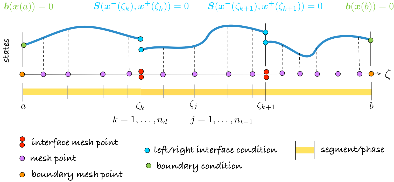
Schematization of Optimal Control Problem formulation with phases.

It is interesting to point out that the boundary condition can be activated or deactivated in runtime, and it is not necessary to regenerate the source code of the project (and recompile) if numerical data is changed.

This feature allows to easily produce many different test by just editing the numerical field of the data. Another characteristic is the use of penalty functions to ensure the bounds of the variables and to facilitate the numerical convergence to a minimum.

Among the various types of conditions there are initial and final point constraints, the extrema of integration are not fixed to a specific interval, but \([a,b]\) can be chosen by the user. The problems solvable with PINS must have the following rigid 2 structure: a fixed interval for the independent variable, no explicit integral constraints like classic bounds from the calculus of the variations,

2

This is not a limitation or a loss of generality as showed next

\[\int_a^b \mathbf{g}(\mathbf{x},\mathbf{u})\mathrm{d}\,\zeta =\mathbf{0}\]

finally, constant parameters are not allowed. Although this seems a limitation on the flexibility of the kind of problems, those difficulties can be easily overcome by some simple changes of variable as shown in examples. Path constraints

\[\mathbf{c}(\mathbf{x}(\zeta),\mathbf{x}(\zeta),\zeta) \leq \mathbf{0}\]

are not explicitly included in the formulation: the inequalities are approximated and included in the Lagrange term by using penalty or barrier functions See Chapter Quick Start for a broader description of the various types of constraints. With the help of the Theorem of Lagrangian Multipliers the OC problem is transformed into an unconstrained problem. Performing the first variation, the necessary conditions for the solution of the problem are obtained and they must satisfy a (multipoint) Boundary Value Problem (BVP).